Last year, when tutoring a student through how ligands interact with the d orbitals of metals center, I was annoyed to realize that there was no easily accessible d orbital viewer with point charges to represent the ligands. This would have greatly helped explain this concept to my student as it shows in 3D, not 2D like all the online resources I was able to find, that different ligand configurations lead to the raising and lowering of orbital energies via the overlap of the ligand with the orbital. While the 2D representations are helpful; not being able to view all of the ligands at once and having to mentally translate it into a 3D representation presented road blocks that just don’t need to be there when teaching this topic. Therefore, I set out to build a d Orbital Viewer in the hopes others will find it useful.
To start off with I needed the d orbitals. For this I used the d orbitals obtained from the solutions to the hydrogen atom available in an analytical form. These solutions are expressed as:

Where 


Instead of translating the spherical coordinates, 


where:

More information about this transformation can be found on Wikipedia here, while more information about arctan2 function used to implement the 
The code implementing the above is:
def hydrogen_den(X,Y,Z):
    R = np.sqrt(X**2+Y**2+Z**2)
    if R == 0:
        return 0
    Theta = np.arccos(Z/R)
    Phi = np.arctan2(Y,X)

    #l=2 m=0
    #wf = 1/(81*sqrt(6*pi))*R**2.*exp(-R/3)*(3*cos(Theta)**2-1)
    #l=2 m=+-1
    #wf = 1/(81*sqrt(pi))*R**2*exp(-R/3)*sin(Theta)*cos(Theta)*exp(1j*Phi)
    wf = 1/(81*sqrt(pi))*R**2*exp(-R/3)*sin(Theta)*cos(Theta)*exp(-1j*Phi)
    #l=2 m=+-2
    #wf = 1/(162*sqrt(pi))*R**2*exp(-R/3)*sin(Theta)**2*exp(2j*Phi)
    #wf = 1/(162*sqrt(pi))*R**2*exp(-R/3)*sin(Theta)**2*exp(-2j*Phi)
    return (wf*np.conj(wf)).real
This function takes in coordinates in cartesian space, converts them to spherical coordinates, calculates the desired 3d orbital based on what wf = is not commented out, and lastly obtains the electronic density by multiplying the resulting wavefunction value by its complex conjugate. To suppress a numpy warning I return just the real part of the result (Although there shouldn’t have been any complex component left anyway).
Strange solutions?
If we were to just view the density of each wavefunction above we’d get these as results:
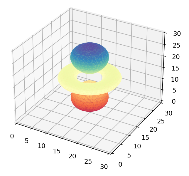 The  orbital orbital |
 The  orbital orbital |
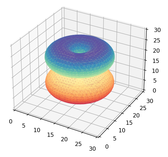 The  orbital orbital |
 The  orbital orbital |
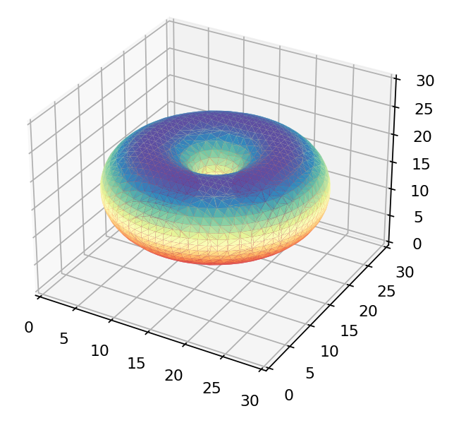 The  orbital orbital |
Only the first of these looks like the 3d orbitals we see in chemistry textbooks as shown below! What’s going on?
As it turns out while the 


Now that we have the usual 3d orbital wavefunctions and can obtain the electron density at any arbitrary coordinate in space its time to start sampling some points!