Building a d Orbital Viewer for 3D Crystal Field Theory Visualization – Part Two: Let’s Visualize Some Orbitals!

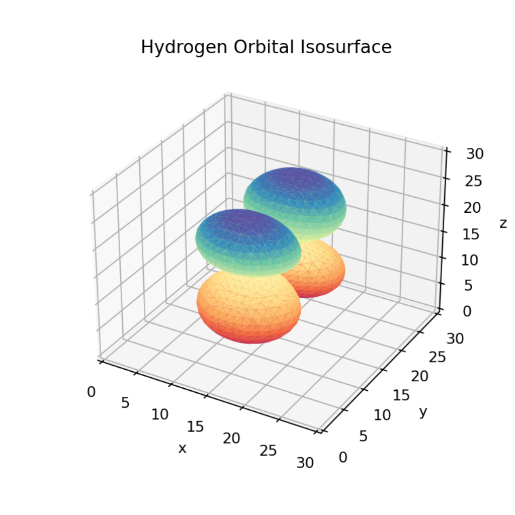
In the previous post we created python code to obtain the value of each 3d orbital’s density at an arbitrary point in space; now we need create a way to view the orbitals in 3D space and generate an isosurface .glb file that can be read by rendering software such as blender or three.js. First we will work on plotting an isosurface using matplotlib before exporting it as a .glb file.

Matplotlib Visualization

As we have code to generate each orbitals density at an arbitrary point in space we now need to sample some points! We can do this by using the arange function within numpy not create arrays of equally spaced values between an upper and lower bound as:

dz = 0
zmin = -15
zmax = 15
x = np.arange(zmin,zmax,dz)
y = np.arange(zmin,zmax,dz)
z = np.arange(zmin,zmax,dz)

Creating a tensor to contain the electron density at every point in the above defined space; we can now iterate through the points calling our previously defined hydrogen_den function to evaluate the density

data = np.zeros((len(x),len(y),len(z)))
for i in range(len(x)):
    for j in range(len(y)):
        for k in range(len(z)):
            data[i][j][k] = hydrogen_den(x[i],y[j],z[k])

Now how do we plot this? We can’t visualize every points density or else we’ll just end up with a graph of all the points colored in based on their value. Instead we can limit our view to a specific value of the orbitals density to create a three dimensional surface to plot. For this I used the skimage’s marching cubes algorithm to generate vertices and faces from the density tensor.

max_val = np.max(data)
verts, faces, _, _ = measure.marching_cubes(data, max_val/6, spacing = (1,1,1))

Here we define the isosurface value to be 1/6^th the maximal value of the density. This can be adjusted to higher or lower if necessary. We also need to define the spacing to match the x,y,z distance between adjacent points. Now that we have the faces and vertices we can actually plot them! It’s

fig = plt.figure()
ax = fig.add_subplot(111, projection='3d')
ax.set_xlim([0,len(x)])
ax.set_ylim([0,len(y)])
ax.set_zlim([0,len(z)])
ax.set_xlabel("x")
ax.set_ylabel("y")
ax.set_zlabel("z")

ax.plot_trisurf(verts[:,0], verts[:,1], faces, verts[:,2], cmap ='Spectral', lw=0)

ax.set_title("Hydrogen Orbital Isosurface")

plt.show()

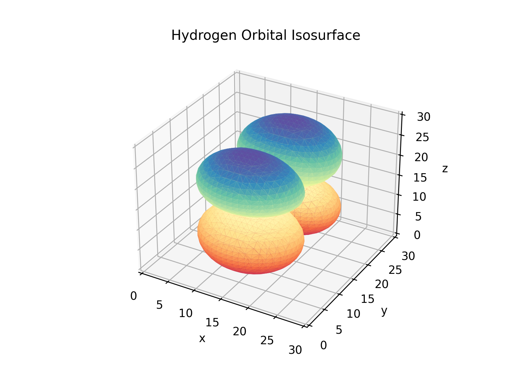
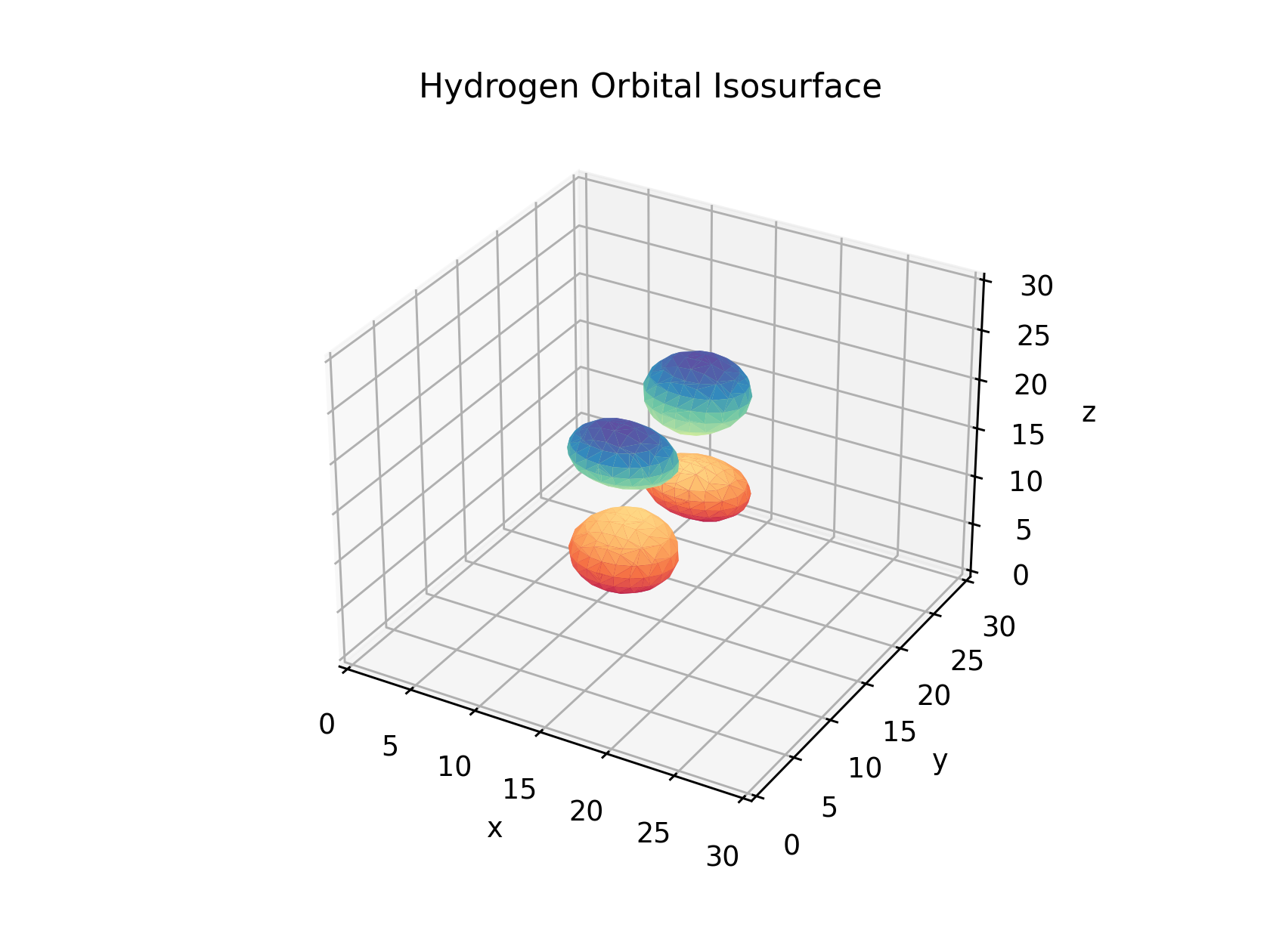
If we adjust the isosurface value to 1/18^th and 1/2 of the maximal value as shows below we can adjust the size of the orbitals we visualize. If you choose values above the maximal value or below the minimal there will be no isosurface produced as their are no values above and below those to define the bounds of the mesh.

Optional: Interactivity

If you want this to be interactive use %matplotlib widget and install the conda install -c conda-forge ipympl

We can add more interactivity to the plot by creating a slider which will adjust the isosurface value in real time. To do this we first need to create a slider which we can interact with the graph through

sli = Slider(plt.axes([0.25, 0.025, 0.65, 0.03]), "iso", 0, max_val, valinit=max_val/2)

Unfortunately with just the slider our code doesn’t actually change anything when the sliders value is adjusted. For this to happen we need to attach a function to the slider such that it is called on a change in value. For this I’ve called the function update which takes in the updated isosurface value and generates a new set of faces and vertices using the marching cubes algorithm and updates the plot. We set the update function to be called when the slider changes by passing it into the sli.on_changed function.

def update(val):
    ax.clear()
    verts, faces,_, _ = measure.marching_cubes(data, val/6, spacing = (1,1,1))
    ax.plot_trisurf(verts[:,0], verts[:,1], faces, verts[:,2], cmap ='Spectral', lw=0)
    ax.set_xlim([0,len(x)])
    ax.set_ylim([0,len(y)])
    ax.set_zlim([0,len(z)])
    ax.set_title("Hydrogen Orbital Isosurface ("+str("%.5f"%sli.val)+")")
           
sli.on_changed(update)